

Experimenting with Time Series and KNIME Nodes
Making use of low-code, open-source models in KNIME to evaluate time series forecasting for pricing estimates

Time series has been one of the most talked about and, arguably, most well-known topics in supply chain management. It has also presented significant opportunities in analytics and, more recently, machine learning fields. It involves analyzing data points over a period of time to forecast future trends and patterns. Beyond seeing their results in supply chain planning platforms, most of us have had limited access to real-world examples where we can actually observe how time-series algorithms can help predict future data points.
Thus, I decided to conduct a mini-experiment to learn the ins and outs of time series modelling and identify the most important pieces of information to gather before beginning the process. As someone who is new to coding and passionate about KNIME, I have chosen to use KNIME as my main tool. I also incorporate Python scripts when necessary for my experiments. In order to figure out what input/critical data points to use, I followed the steps in the KNIME community's published book and looked into the recommendations made by other members online. By diligently following the instructions provided in the KNIME manual and utilising Python scripts when needed, I gained a deeper understanding of time series modelling and developed a clearer awareness of its limitations.
Experiment — You are a data scientist asked to analyze an avocado dataset by your team. The task at hand is to pick a specific avocado type in the whole of the US and forecast its daily average prices.
Approach — Utilize KNIME to carry out data pre-processing and subsequently run the training and test datasets across multiple models to evaluate model quality.
Results — Evaluate the accuracy of different models basis the scoring metrics to observe the effectiveness of different models.
Utilizing KNIME for Data Manipulation and Pre-Processing
The first step in the data cleansing process involves aggregating the data for each individual day, specifically focusing on the “conventional” type within the project data. This task is simplified by utilizing a range of in-built KNIME nodes, which are detailed below.
Exploring the new time series extension nodes can be incredibly beneficial for estimating input parameters like p, d, q, P, D, Q, and s. Utilizing tools such as the Autocorrelation Plot and the Python module for seasonal decomposition allows for experimentation and helps in pinpointing the most suitable value for seasonality (s).
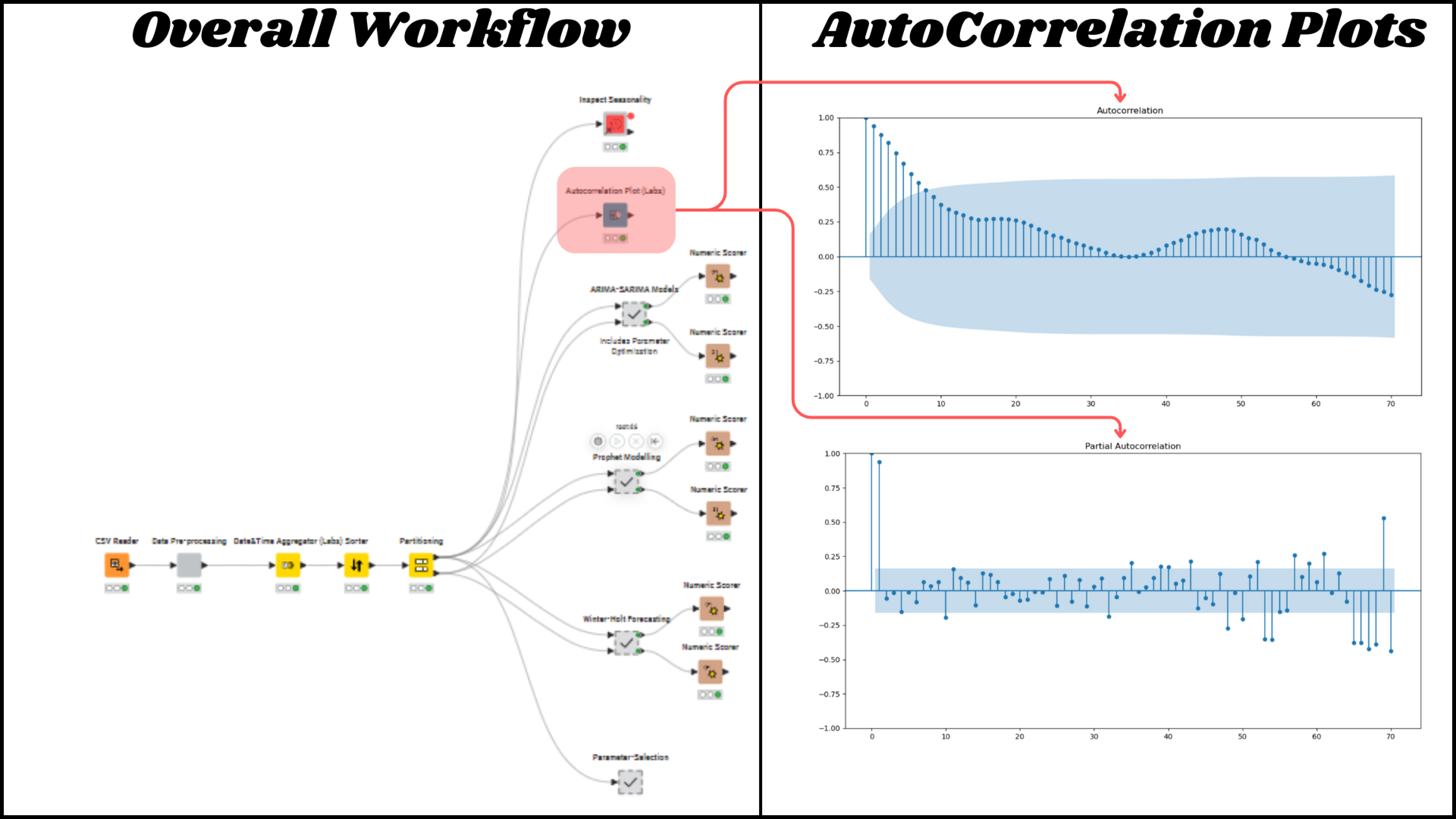
There are a number of articles that provide guidance in terms of identifying the above shared parameters through the use of ACF and PACF plots. I will not go into the details. The Knime ebook Codeless Time Series Analysis with Knime provides good guidance for establishing the parameters but, I would also suggest browsing the internet to improve one’s understanding further.
Running Time Series Modelling with KNIME Nodes
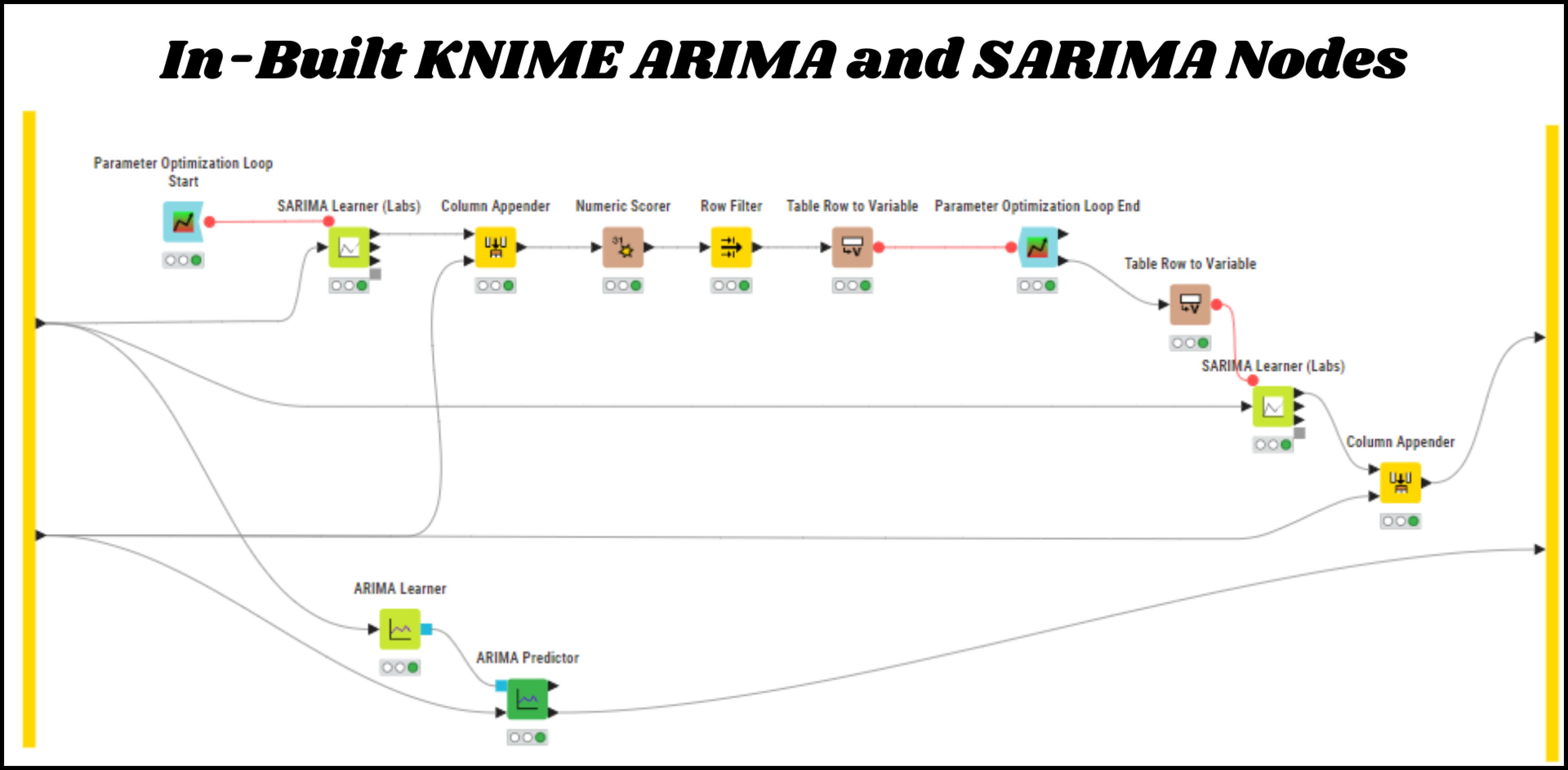
Knime offers a variety of built-in nodes specifically designed for time series modelling, included within its extensions. One of the standout benefits of these nodes is that they enable amateur users, such as myself, to concentrate mainly on the input parameters. This means we can skip the time-consuming task of writing the Python code ourselves.
Imagine the time you could save, particularly if you are not a coding expert! With the ready-made in-built nodes at your disposal, you can dive straight into your analysis without getting bogged down in the technical details.
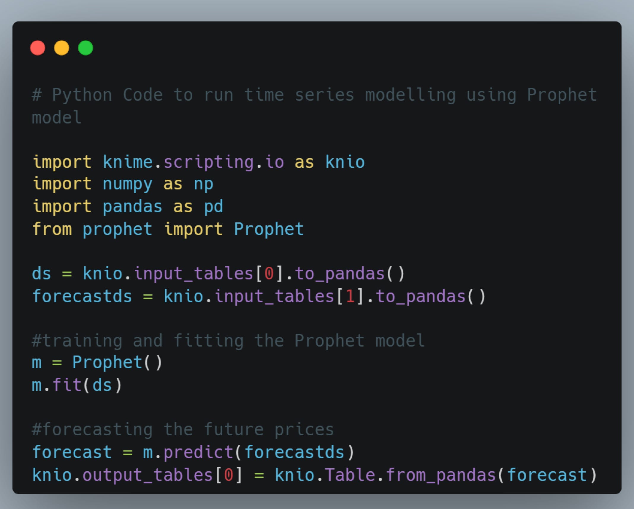
KNIME provides the additional option to write Python code, allowing you to conduct your own tailored analysis. I took advantage of this feature by crafting Pythonic code to execute open-source Prophet, NeuralProphet, and Winter-Holt Smoothing models. This allowed me to assess the performance and forecasting quality of different models, all while staying within the familiar KNIME interface.
A sample code written within the KNIME Python Script node for utilizing the Prophet model is provided below for ease of reference.
A mix of all these capabilities allowed me to experiment with the following list of models for the purpose of my study as shared below —
SARIMA and ARIMA models
Prophet
Neural Prophet
Winter-Holt Smoothening
Model Performance Results and Key Takeaways
Comparing the Mean Absolute Percentage Error for every model created for the "Test" dataset is a crucial method for assessing the quality of the models. KNIME offers the Numeric Scorer node, which is a convenient tool for producing several performance measures, including R^2, RMSE, MAE, and MAPE. I have decided to utilize MAPE as a benchmark for my project in order to assess how well each model performs.
Key Takeaways
Traditional models like SARIMA and ARIMA reported better performance as compared to the other models.
Using pre-built KNIME environments can save a lot of time for business experts, allowing them to focus on business insights rather than backend development activities.
In order to identify a potential solution, it is necessary to experiment with various models and adjust parameters based on the specific business problem, rather than rushing to a hasty conclusion.
A one-size-fits-all approach does not suffice, thus it is crucial to collaborate with Subject Matter Experts, such as Data Scientists and Statisticians, to transform initial prototypes into sophisticated working models that aid businesses in real-time decision-making.
References
Codeless Time Series Analysis with KNIME | KNIME
Why is R^2 Not Used to Measure Time Series Analysis Performance? - YouTube - KNIMETV